Fast(er) 3D Resistive Force Theory
Published:
This is a vectorized implementation of 3D resistive force theory (Agarwal et al., PNAS 2023) with support for custom intruder geometries. You can get the source code from my GitHub repo.
What is Resistive Force Theory?
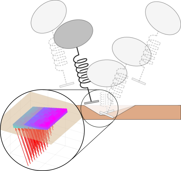
Resistive force theory (RFT) is a numerical method that models the resistive force and torque experienced by an object as it moves through a resistive medium (e.g., a fluid). The fundamental assumption underpinning RFT is that the resistive force and torque (together, the resistive wrench) is the linear superposition of the infinitesimal forces on each element of the intruder’s surface. This is a drastic simplification compared to solving a system of partial differential equations (if they are even known) that model the bulk behavior of the resistive medium in response to the moving intruder.
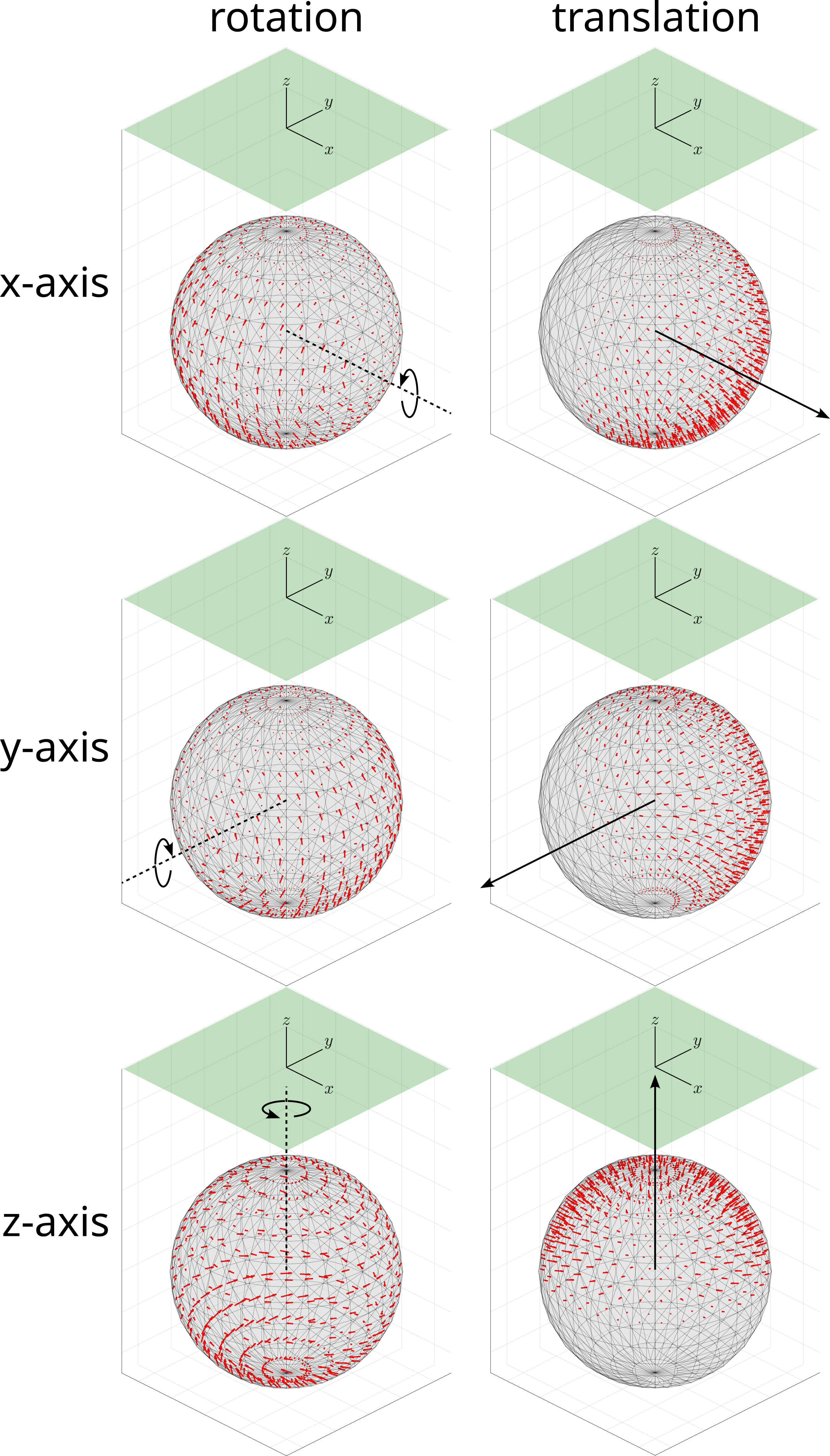
RFT was originally applied to low-Reynolds-number fluids (Gray and Hancock, JEB, 1955) but, more recently, it has turned out to work quite well for granular media. So-called granular RFT was first developed for planar motion (Li et al., Science, 2013) and, more recently, for three-dimensional motion (Agarwal et al., PNAS 2023).
RFT maps the intruder configuration and twist to a resistive wrench and is parameterized by the intruder geometry as well as a set of coefficients (typically obtained empirically by fitting to data):
\(\mathcal{F}_\mathrm{f} = \mathrm{RFT}\left(T_\mathrm{wf},\mathcal{V}_\mathrm{f};\texttt{geom},C\right),\) where
- \(\mathcal{F}_\mathrm{f}\in\mathbb{R}^6\) is the resistive wrench expressed in the intruder frame \(\{\mathrm{f}\}\); \(\mathcal{F}_\mathrm{f} = \left[\tau_\mathrm{f}^\top,f_\mathrm{f}^\top\right]^\top\), where \(\tau_\mathrm{f}\in\mathbb{R}^3\) is the resistive torque in \(\{\mathrm{f}\}\) and \(f_\mathrm{f}\in\mathbb{R}^3\) is the resistive force in \(\{\mathrm{f}\}\);
- \(T_\mathrm{wf}\in\mathsf{SE}(3)\) is the configuration of the intruder frame \(\{\mathrm{f}\}\) relative to the world frame \(\{\mathrm{w}\}\), where \(R_\mathrm{wf}\in\mathsf{SO}(3)\) is the orientation of \(\{\mathrm{f}\}\) relative to \(\{\mathrm{w}\}\) and \(p_\mathrm{wf}\in\mathbb{R}^3\) is the position of \(\{\mathrm{f}\}\) relative to \(\{\mathrm{w}\}\);
- \(\mathcal{V}_\mathrm{f}\in\mathbb{R}^6\) is the intruder twist expressed in \(\{\mathrm{f}\}\); \(\mathcal{V}_\mathrm{f} = \left[\omega_\mathrm{f}^\top,v_\mathrm{f}^\top\right]^\top\), where \(\omega_\mathrm{f}\in\mathbb{R}^3\) is the angular velocity in \(\{\mathrm{f}\}\) and \(v_\mathrm{f}\in\mathbb{R}^3\) is the linear velocity in \(\{\mathrm{f}\}\);
- \(\texttt{geom}\) is some description of the intruder geometry, for example a triangulation object (i.e., a polyhedral graph) \(\texttt{TR} = \left(\texttt{V},\texttt{E}\right)\) consisting of \(N\) vertices \(\texttt{V}\) and \(M\) edges \(\texttt{E}\);
- \(C\in\mathbb{R}^{m\times 3}\) is a set of \(m\) 3-vector-valued coefficients that relate the local traction force (also a 3-vector) on a face of the intruder to the orientation of the face, the direction in which it moves, and the direction in which gravity acts.
RFT can be interpreted as convolution, where the convolution kernel is a map from the kinematics of an individual surface element to the resistive traction force on the element. The approach taken by Agarwal et al. beautifully exploits symmetries (invariance, equivariance) in the physics to reduce the relevant local kinematics to three unit vectors:
- \(\hat{n}^i\), the outward-pointing unit vector normal to surface element \(i\);
- \(\hat{v}^i\), the direction in which surface element \(i\) is moving (instantaneously);
- \(\hat{g}\), the direction in which gravity points.
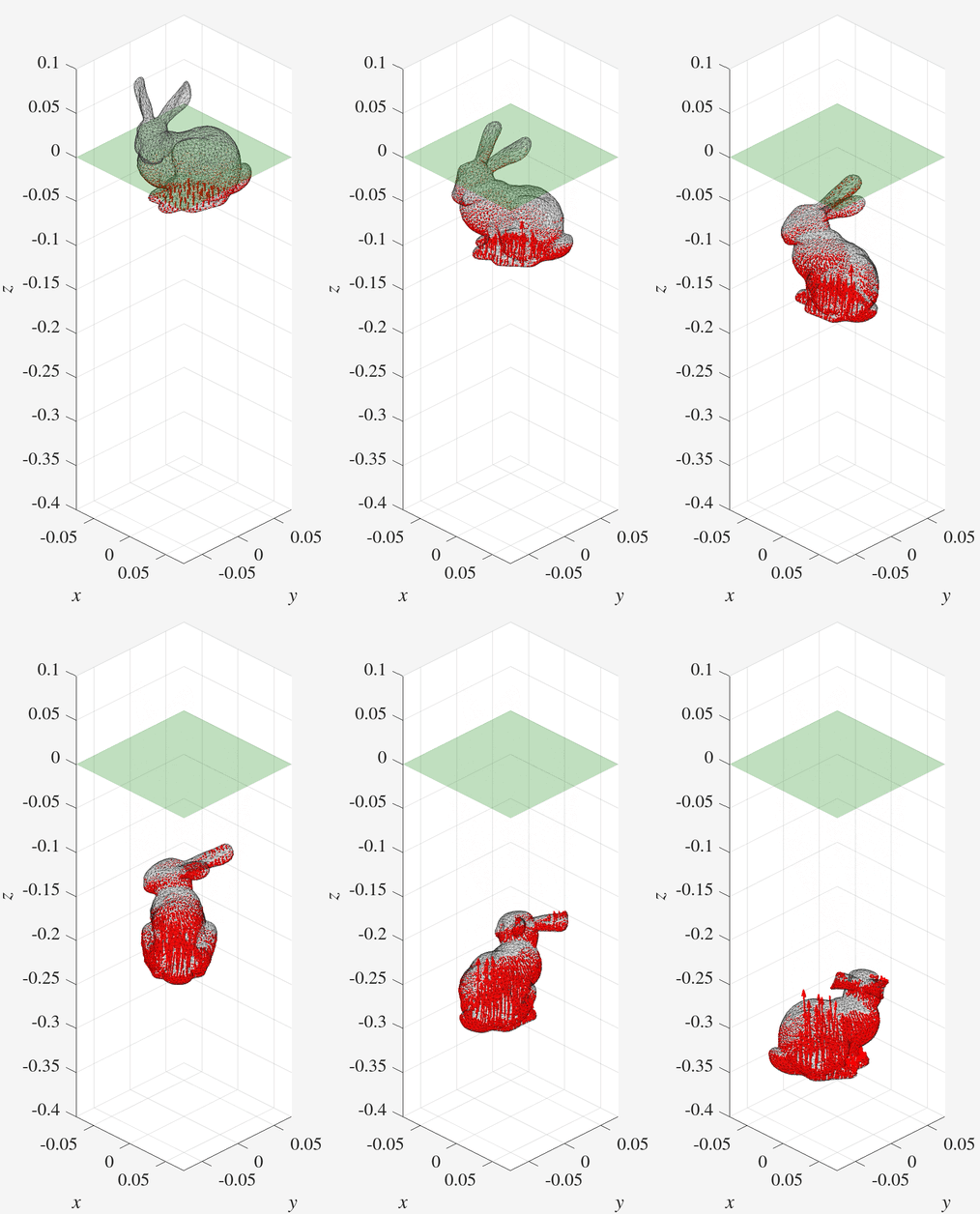
The diagram below depicts these unit vectors, and the predicted resistive traction vector \(f^i\), for an individual surface element of an intruder (the Stanford bunny) moving with twist \(\mathcal{V}\).
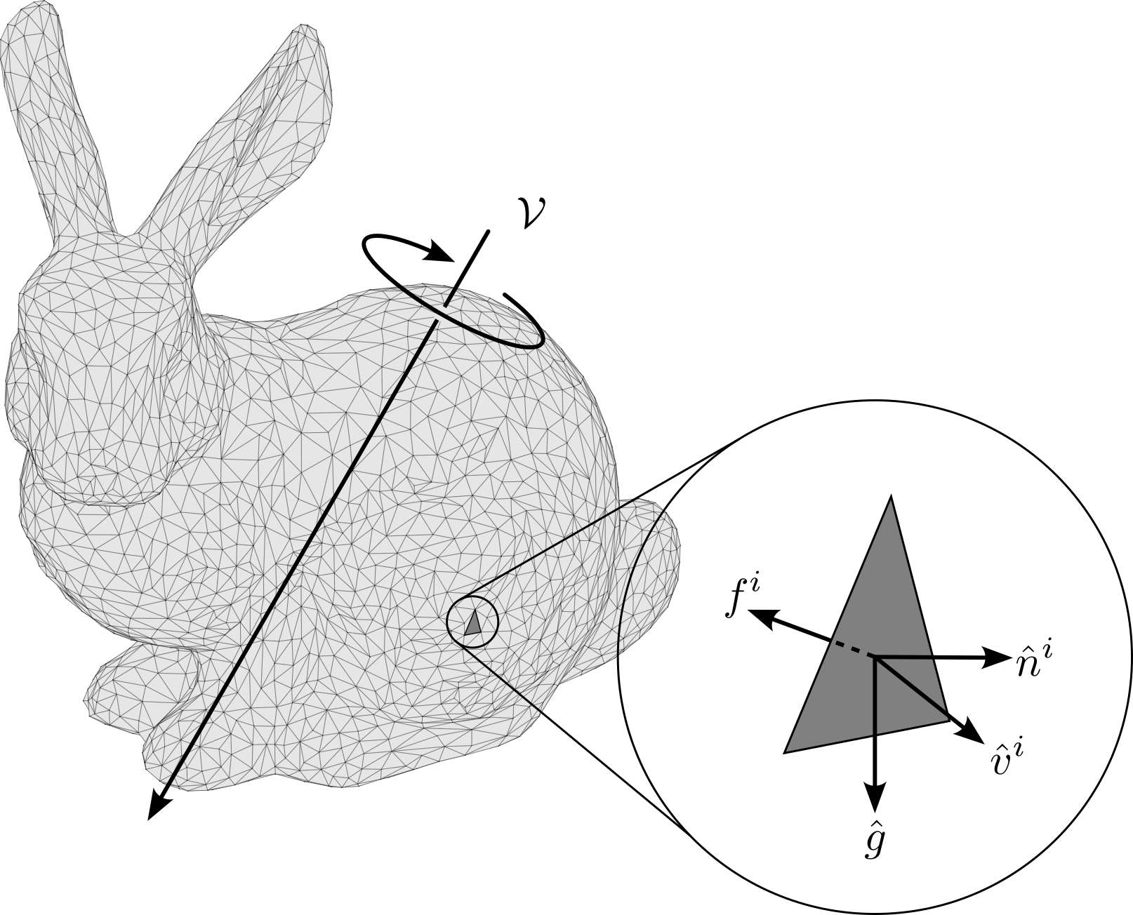
If the element is not submerged, then \(f^i = 0\). Also, if the element is not moving “into” the medium, i.e., if \(\hat{n}^i\cdot\hat{v}^i \leq 0\), then \(f^i = 0\) (this is called the “leading-edge” or “leading-face” hypothesis). Otherwise, \(f^i\) is scaled by the element depth, its area, and a coefficient that parameterizes the medium’s penetration resistance (measured in stress per unit depth).
What’s Special about My Implementation?
It’s (relatively) fast. I recognized that the algorithm published by Agarwal et al. depends on the dot products between three unit vectors and not on the directions of the vectors themselves. This is great for two reasons:
- Working exclusively in terms of dot products bypasses several artificial edge cases that arise from using angles to describe the orientation of one vector relative to another. Computationally, there’s no need to use if-else logic to check these edge cases, and there’s no trigonometry required.
- As a result, the RFT algorithm reduces to matrix-vector operations.
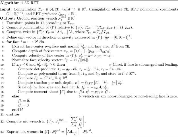
A consequence of the second point is that the algorithm can be implemented using array programming (vectorization), resulting in a significant speedup. My implementation, available on GitHub, uses vectorization; for ease of reading, though, here is what the algorithm looks like using a for loop: