Rigid-Body Mechanics on SE(3) with Impacts

This simple project combines a geometric integrator and event detection to simulate an American football (or a rugby ball!) tumbling through the air and bouncing on a hard surface.

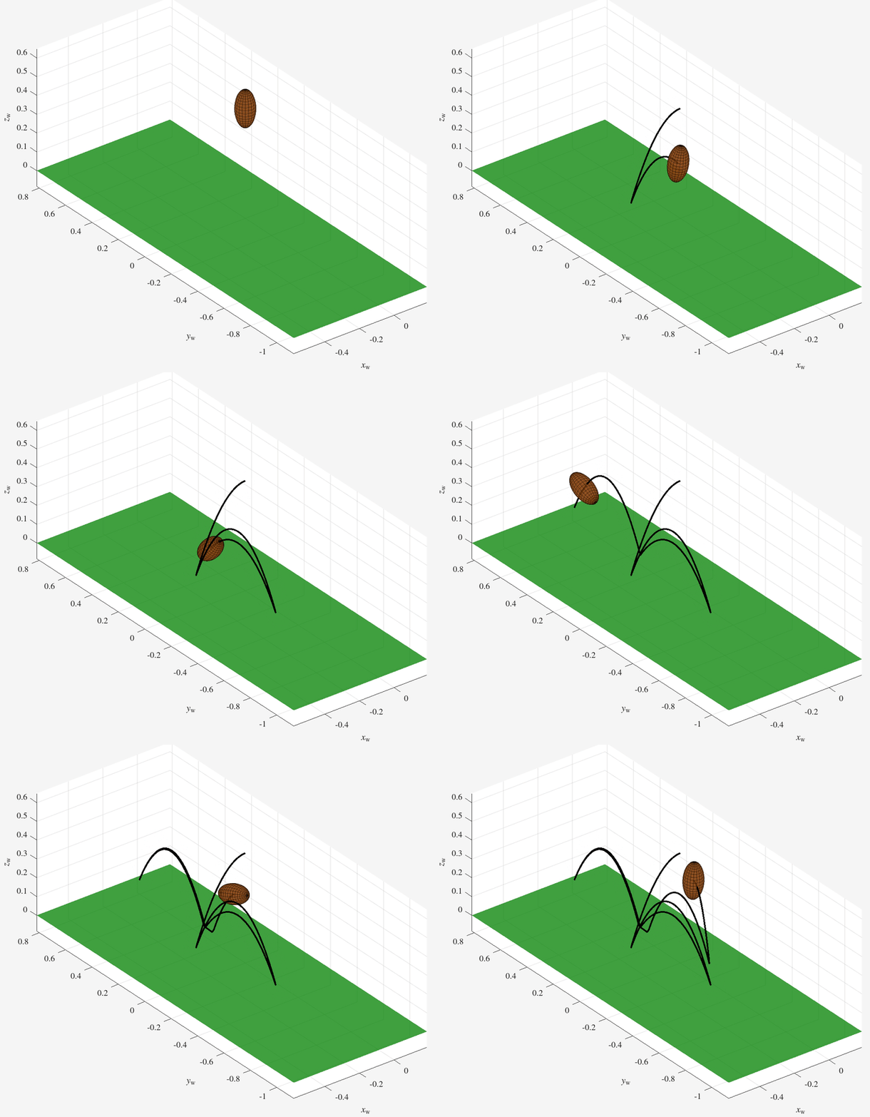
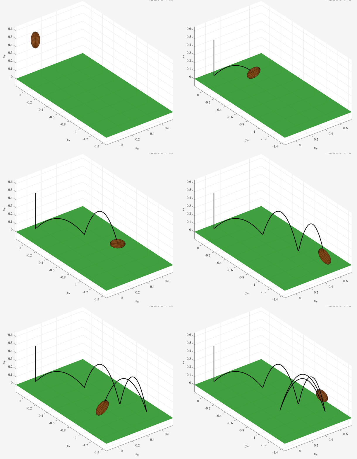
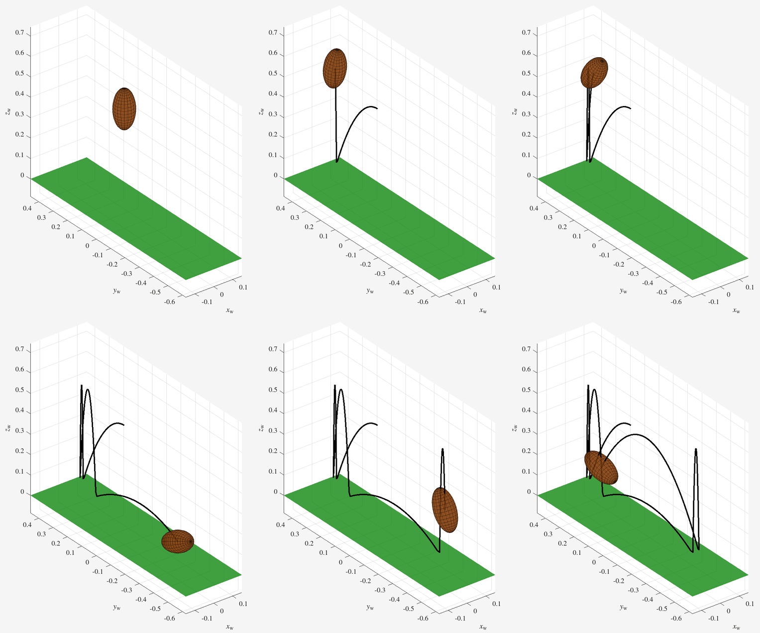
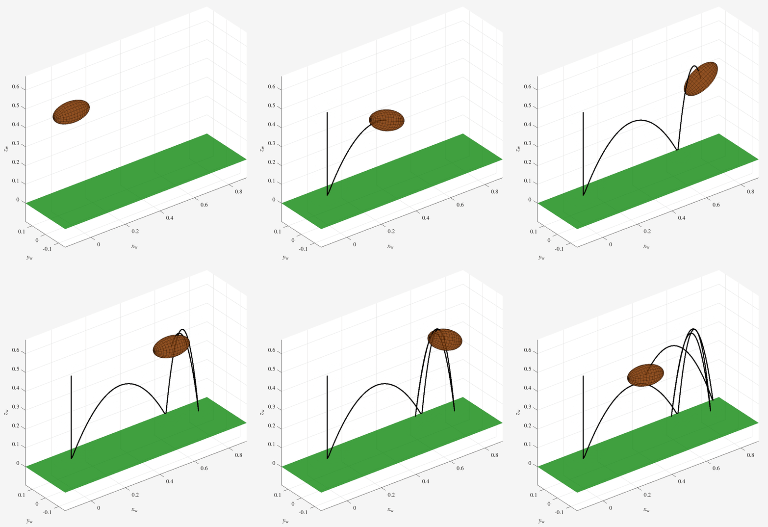
You can get the source code from my GitHub repo.

This toy problem is a good application for so-called geometric integrators that respect the (possibly non-Euclidean) geometry of the relevant physics (rigid-body mechanics, in this case), by evolving the system configuration directly on the configuration manifold (the matrix Lie group \(\mathsf{SE}(3)\), in this case) without relying on one or more charts of local coordinates (e.g., Euler angles). Anyone who has tried to chase and catch a bouncing football knows that it tumbles and bounces wildly, so it’s unlikely that a single coordinate chart will be sufficient for representing the ball’s configuration for all time.

Geometry of Rigid-Body Mechanics

I find the modern differential-geometric approach to rigid-body mechanics fascinating, although I will be the first to admit that what I know is vastly outweighed by what I don’t know.

Geometrically, the state space of a rigid body moving in three-dimensional space is the tangent bundle \(\mathsf{TSE}(3)\), i.e., the union of tangent spaces \(\mathsf{T}_{T}\mathsf{SE}(3)\) over all configurations \(T\in\mathsf{SE}(3)\). We can always multiply a tangent vector \(\dot{T}\in\mathsf{T}_{T}\mathsf{SE}(3)\) by \(T^{-1}\), either by left-multiplication or right-multiplication, to bring it back to the tangent space at the identity \(\mathsf{T}_{I}\mathsf{SE}(3) \cong \mathfrak{se}(3)\); multiplying \(T^{-1}\dot{T}\) is called left-trivialization, and multiplying \(\dot{T} T^{-1}\) is called right-trivialization. Left-trivialization and right-trivialization allow us to identify the tangent bundle \(\mathsf{TSE}(3)\) with \(\mathsf{SE}(3)\times\mathfrak{se}(3)\). Conveniently, \(\mathfrak{se}(3)\) is isomorphic to \(\mathbb{R}^6\), the space of twists. Thus, we interpret the state space as \(\mathsf{SE}(3)\times\mathbb{R}^6\), so the state of the rigid body consists of its configuration \(T\in\mathsf{SE}(3)\) and its twist \(\mathcal{V}\in\mathbb{R}^6\). Left-trivialization leads to body twists: \(\mathcal{V}_\mathrm{b} \cong \hat{\mathcal{V}}_\mathrm{b} \triangleq T_\mathrm{wb}^{-1}\dot{T}_\mathrm{wb}\), and right-trivialization leads to spatial twists: \(\mathcal{V}_\mathrm{w} \cong \hat{\mathcal{V}}_\mathrm{w} \triangleq \dot{T}_\mathrm{wb}T_\mathrm{wb}^{-1}\). The remainder of this portfolio entry deals with left-trivialization; the approach for right-trivialization is essentially the same.

The left-trivialized equations of motion (i.e., equation of motion in the body frame) for a single rigid-body moving in three-dimensional space under the influence of gravity are

where

• \(T_\mathrm{wb}\in\mathsf{SE}(3)\) is the configuration of the body’s center-of-mass (COM) frame \(\{\mathrm{b}\}\) relative to the inertial world frame \(\{\mathrm{w}\}\);
• \(\hat{\mathcal{V}}_\mathrm{b}\in\mathfrak{se}(3)\) is the matrix representation of the body twist \(\mathcal{V}_\mathrm{b}\in\mathbb{R}^6\), where \(\mathcal{V}_\mathrm{b} = \left[\omega_\mathrm{b}^\top,v_\mathrm{b}^\top\right]^\top\), where \(\omega_\mathrm{b}\in\mathbb{R}^3\) and \(v_\mathrm{b}\in\mathbb{R}^3\) are the angular and linear velocity, respectively, of \(\{\mathrm{b}\}\) expressed in \(\{\mathrm{b}\}\);
• \(\mathcal{G}_\mathrm{b}\in\mathbb{R}^{6\times 6}\) is the body’s generalized inertia tensor; \(\mathcal{G}_\mathrm{b}\) is a diagonal matrix with \(\left(\mathcal{I}_\mathrm{xx},\mathcal{I}_\mathrm{yy},\mathcal{I}_\mathrm{zz},m,m,m\right)\) along the diagonal, where \(\left(\mathcal{I}_\mathrm{xx},\mathcal{I}_\mathrm{yy},\mathcal{I}_\mathrm{zz}\right)\) are the moments of inertia about the principal axes and \(m\) is the body’s mass;
• \(\left[\mathrm{ad}_{\mathcal{V}_\mathrm{b}}\right]\in\mathbb{R}^{6\times 6}\) is the adjoint representation of the body twist \(\mathcal{V}_\mathrm{b}\):

\(\left[\mathrm{ad}_{\mathcal{V}_\mathrm{b}}\right]\in\mathbb{R}^{6\times 6} = \begin{bmatrix} \hat{\omega}_\mathrm{b} & 0_{3\times 3}\\ \hat{v}_\mathrm{b} & \hat{\omega}_\mathrm{b} \end{bmatrix},\) where \(\hat{\omega}_\mathrm{b}\) and \(\hat{v}_\mathrm{b}\) are 3-by-3 skew-symmetric matrix representations of the body-frame angular velocity \(\omega_\mathrm{b}\in\mathbb{R}^3\) and linear velocity \(v_\mathrm{b}\in\mathbb{R}^3\), respectively;

• \(\mathcal{F}_\mathrm{b}^\mathrm{grav}\in\mathbb{R}^6\) is the wrench on the body, expressed in \(\{\mathrm{b}\}\), due to gravity:

\(\mathcal{F}_\mathrm{b}^\mathrm{grav} = \begin{bmatrix} R_\mathrm{wb}^\top & 0_\mathrm{3\times 3}\\ 0_\mathrm{3\times 3} & R_\mathrm{wb}R_\mathrm{wb}^\top \end{bmatrix} \begin{bmatrix} 0_{5\times 1}\\ -m g \end{bmatrix},\) where \(g\) is the acceleration due to gravity.

To simulate the bouncing rigid body without first choosing local coordinates, we use a geometric integrator.

Choosing a geometric integrator

There are many kinds of geometric integrators in the literature. Park and Chung wrote a nice review comparing three integrators: Crouch-Grossman, commutator-free, and Munthe-Kaas. For this project, I used a 4th-order 5-stage Crouch-Grossman integrator (CG4), which essentially generalizes the standard 4th-order Runge-Kutta integrator (RK4) to manifolds. Crouch-Grossman integrators were among the first geometric integrators to be developed, and more recent geometric integrators, including variational integrators, may have lower computational complexity and superior long-term energy/momentum conservation, but CG4 is a good starting point because it so closely resembles RK4.

Crouch-Grossman integrators use the exponential map from \(\mathfrak{se}(3)\) to \(\mathsf{SE}(3)\) to step the configuration forward in time and use addition on \(\mathbb{R}^6\) to step the body twist forward in time. The \(s\)-stage Crouch-Grossman integrator algorithm is listed below.

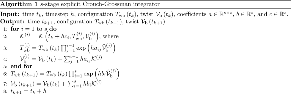
The integrator coefficients \(a_{ij}\), \(b_{i}\), and \(c_{i}\) are listed in the Butcher tableau below.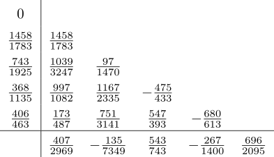

In the s-stage CG integrator algorithm, \(\mathcal{K}\left(t,T_\mathrm{wb},\mathcal{V}_\mathrm{b}\right)\) is an abbreviation for the forward dynamics of the rigid body:

The “post-product operator” used in lines 3 and 6 of the algorithm is defined as follows, for any sequence of square matrices \(A_k\):

Impacts

The animation above also shows impacts. To handle impacts, you need three things:

1. Impact kinematics
2. Impact detection
3. Impact update

Impact kinematics

An impact occurs when the distance between the ground and the nearest point on the ellipsoid goes to zero.

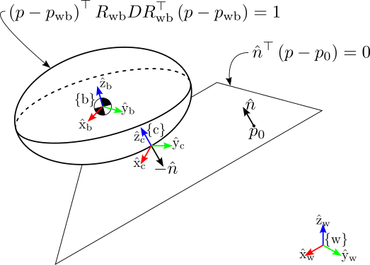
The ellipsoid is defined by the implicit equation

where \(p\in\mathbb{R}^3\), \(\left(R_\mathrm{wb},p_\mathrm{wb}\right)\in\mathsf{SE}(3)\), and \(D\in\mathbb{R}^{3\times 3}\) is a diagonal matrix whose entries are the reciprocals of the squares of the ellipsoid semiaxes. This equation can be written more concisely as

where \(q = \left(p - p_\mathrm{wb}\right)\) and \(A = R_\mathrm{wb} D R_\mathrm{wb}^\top\). By construction, then, \(A\) is symmetric and the ellipsoid is an affine transformation of the sphere. A corollary of all this is that the unit vector normal to the surface of the ellipsoid at the point \(q\) furthest in some \(\hat{e}\)-direction is simply \(\hat{e}\). The matrix \(A\) stretches the vector \(q\) by some amount \(\mu\) and rotates it to align with \(\hat{e}\):

Solving for \(q\), we have

Substituting this result into the (simplified) implicit ellipsoid equation, we have

Solving for the scaling factor \(\mu\), we get

so

The ground is modeled as a plane, defined implicitly by a point \(p_0\in\mathbb{R}^3\) and a unit normal vector \(\hat{n}\in\mathbb{R}^3\), both expressed in the world frame \(\{\mathrm{w}\}\):

For example, when \(p_0 = \left[0,0,0\right]^\top\) and \(\hat{n} = \left[0,0,1\right]^\top\), the ground is simply the x-y plane in the world frame.

To find the point \(c\in\mathbb{R}^3\) on the ellipsoid closest to the ground plane, we substitute \(-\hat{n}\) for \(\hat{e}\) and \(c - p_\mathrm{wb}\) for \(q\) in the equation above, and solve for \(c\):

Impact detection

An impact (or, more generally, any “event” in numerical integration terminology) is defined as the zero-crossing of an event function \(h:\mathsf{SE}(3)\times\mathbb{R}^6\to\mathbb{R}\), where \(\mathsf{SE}(3)\times\mathbb{R}^6\) is the left-trivialized state space, using the isomorphism between \(\mathfrak{se}(3)\) and \(\mathbb{R}^6\).

When the event in question is impact, the event function is the signed distance between the nearest point \(c\) on the ellipsoid and the ground plane and is therefore a function of the configuration \(T_\mathrm{wb}\) only:

Impact occurs when \(h = 0\). Zero-crossings are detected using the simple bisection method summarized below in Algorithm 2.

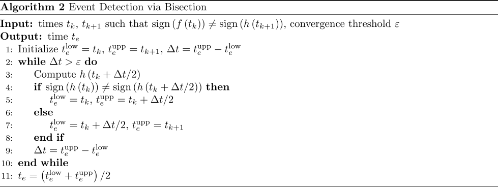
For this method to work, the event function \(h\) must be evaluated at each timestep \(t_k\) for \(k = 1,2,\ldots\) during simulation. A bisection search is executed when the sign of \(h\) changes from \(t_k\) to \(t_{k+1}\).

If the bisection algorithm detects an impact event, the system state must change according to the impact update, described below, after which integration resumes.

Impact update

At impact, there are two kinds of forces at play: there is a normal force and a tangential force; the tangential force arises from Coulomb friction. In general, a contact can be sticking or sliding: in a sticking contact, tangential velocity at the contact point vanishes, and the net contact force lies inside the Coulomb friction cone; in a sliding contact, tangential velocity at the contact point does not vanish, and the net contact force lies on the edge of the friction cone. For simplicity’s sake, I take the friction cone to be the entire half-plane, corresponding to an infinite coefficient of friction—I’d like to relax this assumption when I get the chance to revisit this project in the future, but for now I’ll stick with it.

In rigid-body mechanics, bodies do not deform on impact, impact is instantaneous, and velocities are allowed to undergo jump discontinuities. Thus, instead of considering contact forces acting over a finite contact duration, we consider contact impulses. Upon impact, the ellipsoid experiences an impulse \(\mathcal{J}_\mathrm{c}\in\mathbb{R}^3\). The following constraints hold (instantaneously) at impact:

• the component of the post-impact velocity \(v_{\mathrm{c}}^+\in\mathbb{R}^3\) at the contact point \(c\) normal to the ground plane is related to the pre-impact velocity \(v_{\mathrm{c}}^-\) at the same point by \(v_{\mathrm{c},\perp}^+ = -\varepsilon v_{\mathrm{c},\perp}^-\), where \(v_{\mathrm{c},\perp} \triangleq \hat{n}^\top v_\mathrm{c}\) and \(\varepsilon\in\left[0,1\right]\) is the coefficient of restitution;
• the components of \(v_{\mathrm{c}}^+\) tangent to the ground plane are zero These three constraints on \(v_{\mathrm{c}}^+\) enable us to solve for \(\mathcal{J}_\mathrm{c}\).

Note the contact impulse \(\mathcal{J}_\mathrm{c}\) can be expressed as a linear combination of the feasible impulses directions in \(\{\mathrm{c}\}\):

where

The impulse coefficients \(\lambda\) are given by

where

and

Finally, we compute the contact impulse in \(\{\mathrm{b}\}\):

and then the post-impact body twist